Background
Notations
Let denote the exposure of interest, taking values and . Let be the outcome, the mediator, the time-varying confounder, and the vector of pre-exposure (time-fixed) covariates.
Let and denote the values of the outcome and mediator, respectively, that would have been observed had the exposure been set to ; similarly, and represent the potential values under .
The average total effect can be then decomposed into natural direct and indirect effects as:
The potential outcomes and represent the values of the outcome under exposure levels and , respectively, with the mediator taking its natural value under each exposure. In contrast, describes the outcome under exposure , but with the mediator set to the value it would have taken under , capturing a cross-world scenario relevant to mediation analysis.
In the context of mediator–outcome confounders being affected by the exposure (i.e., $Y_{am} \not\!\perp\!\!\!\perp M_{a^*}|V$ - violation of identification condition), the natural direct and indirect effect above are not identified. The randomized interventional analogues were introduced.
Let denote the a random draw from the distribution of the mediator with exposure is set at conditional on covariates . In other words, reflects a stochastic draw from its conditional distribution rather than a fixed potential value of the mediator. The randomized interventional analogues of natural direct and indirect effects are defined as
In the longitudinal setting, the overbars denote the history of variables up to time . The total effect of a longitudinal exposure regime versus can be decomposed as:
As shown by VanderWeele and Tchetgen Tchetgen (2017), the interventional analogues of natural direct and indirect effects, under the causal DAG (below) where the mediator precedes the time-varying confounder ( preceding ), can be identified using the so-called mediational g-formula.
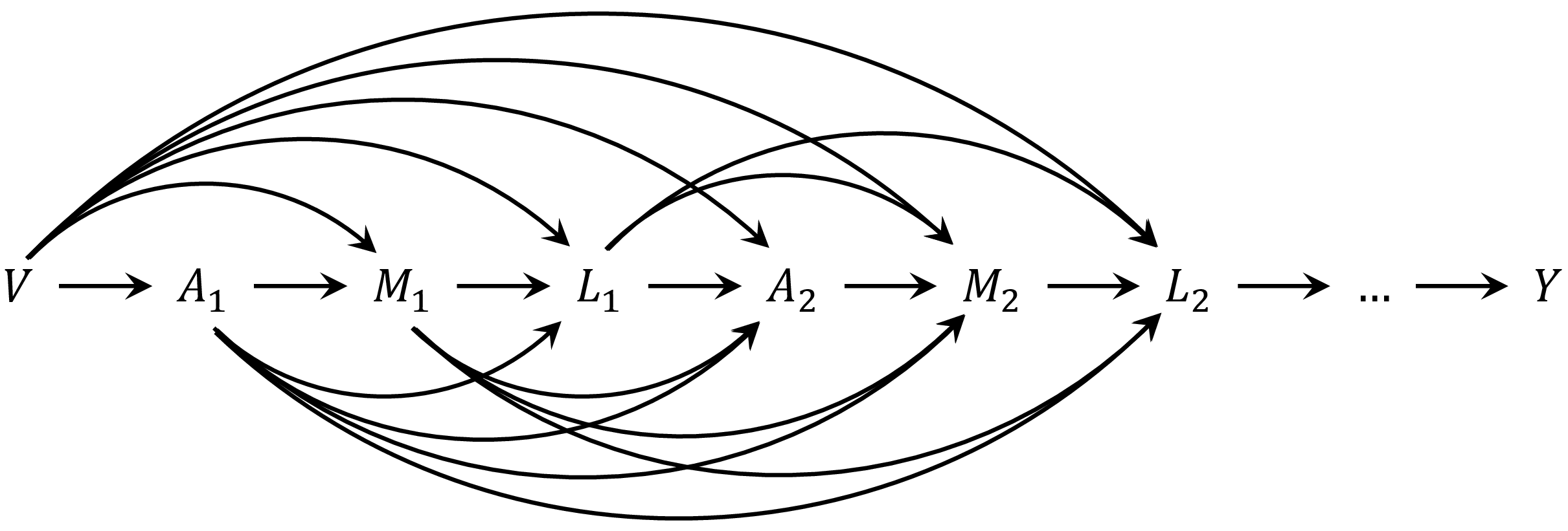
DAG for the context that the mediator precedes the time-varying confounder
In particular, the identification of is
In the context where time-varying confounder precedes the mediator ( preceding )
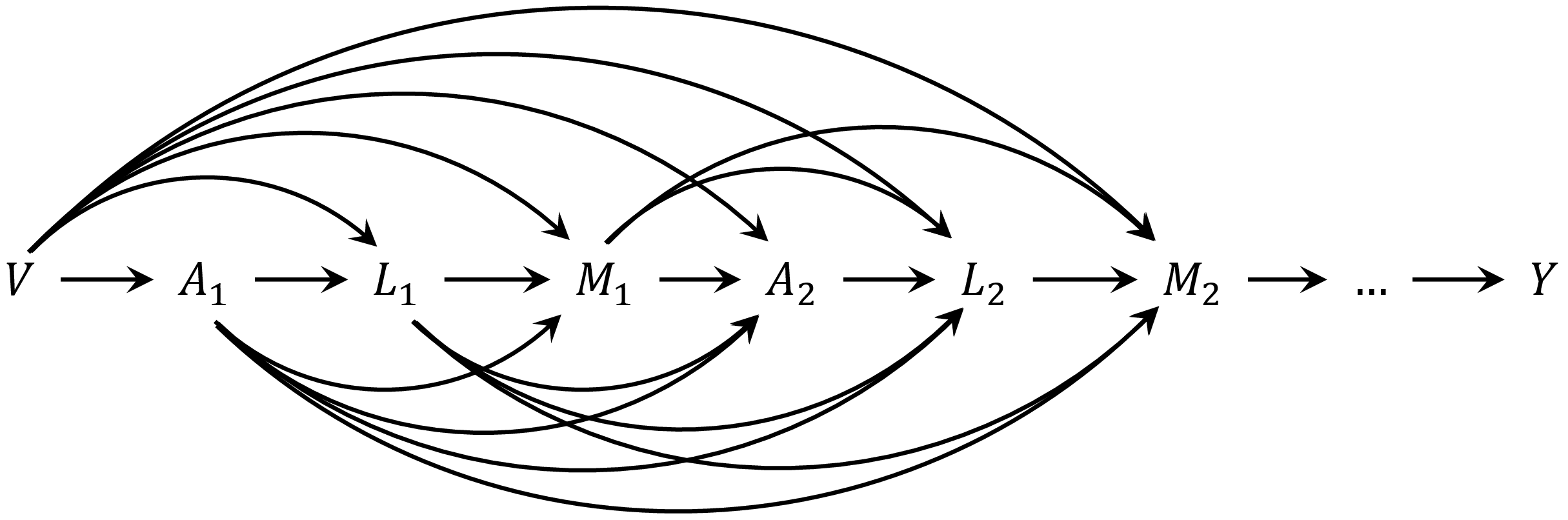
DAG for the context that the time-varying confounder precedes the mediator
The mediational g-formula identification for becomes
For ease of notation, let’s adopt the same shorthand notations as in the VanderWeele and Tchetgen Tchetgen (2017) paper: to represent , for , and for ,
G-computation Algorithms in tvmedg
tvmedg implements g-computation to estimate interventional direct and indirect effects in longitudinal settings, based on the mediational g-formula mentioned above. The core algorithm involves 4 main steps:
-
Step 1: Fitting parametric models
tvmedg()fits the user-specified regression models for each time-varying variable, conditional on relevant history and baseline covariates:- Time-varying confounders:
-
if
(
preceding
)
- if ( preceding )
-
if
(
preceding
)
- Mediator:
- Outcome:
- Time-varying confounders:
Step 2: Monte Carlo sampling
Resample the values of all variables at baseline, including time-fixed covariates and time-varying confounders at time . This step approximates the baseline covariate distribution and improves the stability and precision of predictions in Step 3.Step 3: Predict follow-up
Using the baseline samples generated in Step 2, Step 3 simulates follow-up trajectories by sequentially predicting time-varying confounders, mediators, and outcomes under specified exposure regimes. This process is illustrated in the following figure (as an example for estimating ) in the context of binary outcome.
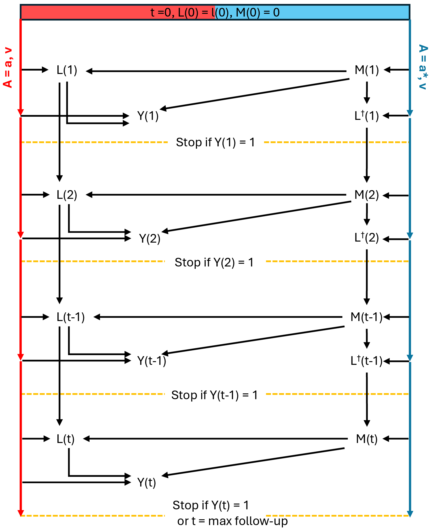
g-computation in tvmedg
-
Step 4: Estimating interventional analogues of natural direct and indirect effects
Estimating , , and at the end of follow-up and derive:Interventional total effect (rTE):
Interventional direct effect (rDE):
Interventional indirect effect:
Proportional explain: Indirect effect / Total effect
References
VanderWeele, T. (2015). Explanation in causal inference: methods for mediation and interaction. Oxford University Press.
VanderWeele, T. J., & Tchetgen Tchetgen, E. J. (2017). Mediation analysis with time varying exposures and mediators. Journal of the Royal Statistical Society Series B: Statistical Methodology, 79(3), 917-938.