Time-varying Mediation Analysis with Binary Exposure and Single Mediator • tvmedg

This example illustrates how to use tvmedg() function to conduct time-varying mediation analysis with binary exposure, single binary mediator, and binary outcome. We will use simulated monthly longitudinal data, where each row represents one month of follow-up per individual. The dataset includes the following variables:

Exposure: $Ap$
Mediator: $Mp$
Outcome: $Yp$
Time-varying confounders: $L_1$ binary, $L_2$ and $L_3$ continuous
Time-fixed confounders: age, sex, ow, and risk
Time index: mm, indicating the month of follow-up

Since, g-computation is computationally intensive, we will leverage parallel computing using the foreach and doParallel packages to improve efficiency

library(tvmedg)
head(sim_data)
#>   id mm Ap Mp L1       L2        L3 Yp      age sex ow risk lastid
#> 1  1  1  0  0  0 100.0000  80.00000  0 16.52949   0  0    0      0
#> 2  1  2  0  0  0 125.1296 102.02885  0 16.52949   0  0    0      0
#> 3  1  3  0  0  0 116.4990  98.99688  0 16.52949   0  0    0      0
#> 4  1  4  0  0  0 131.9247 104.07117  0 16.52949   0  0    0      0
#> 5  1  5  0  0  0 109.5959 103.24813  0 16.52949   0  0    0      0
#> 6  1  6  0  0  0 124.2403  95.82793  0 16.52949   0  0    0      0

Point estimates

First example is when the mediator precedes the time-varying confounders ( $M \rightarrow L$ ). This corresponds to the following DAG

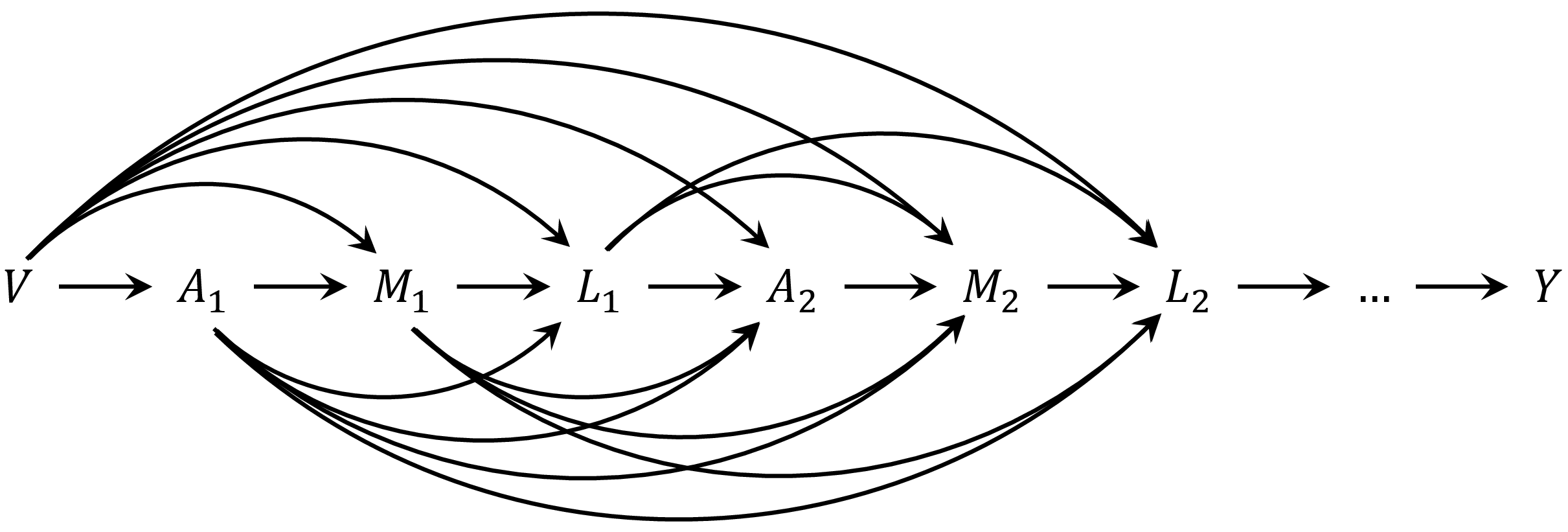
DAG for the context that mediator precedes the time-varying confounders

To specify the causal ordering $M \rightarrow L$ , set the argument tvar_to_med = FALSE (the default). In contrast, if the time-varying confounder is assumed to precede the mediator ( $L \rightarrow M$ ), use tvar_to_med = TRUE.

The current version of tvmedg supports lag-based functional forms for variable histories. In this example, we specify 2 lags. By default, logistic regression is used for binary variables, and linear regression is used for continuous variables. For continuous variables and time indices, spline-based models can be used by specifying: sp_list, sp_type, and sp_df. This example sets a cubic spline with 3 degrees of freedom for the month variable mm. Additional variables, spline types (e.g., “ns”), and df can be added to these arguments to model nonlinear effects. Lastly, we run the algorithm using 1000 Monte Carlo samples.

library(doParallel)
#> Loading required package: foreach
#> Loading required package: iterators
#> Loading required package: parallel

cl <- makeCluster(2)
registerDoParallel(cl)
med_MtoL <- tvmedg(data = sim_data,
                   id = "id",
                   basec = c("age","sex","ow","risk"),
                   expo = c("Ap"),
                   med = c("Mp"),
                   tvar = c("L1","L2","L3"),
                   outc = c("Yp"),
                   time = c("mm"),
                   lag = 2,
                   tvar_to_med = F,
                   cont_exp = F,
                   mreg = "binomial",
                   lreg = c("binomial","gaussian","gaussian"),
                   yreg = "binomial",
                   sp_list = c("mm"),
                   sp_type = c("bs"),
                   sp_df = c(3),
                   followup = 12,
                   seed = 123,
                   montecarlo = 1000,
                   boot = F,
                   parallel = TRUE)
#> Q(a,a): 0.23 
#> Q(a,a*): 0.045 
#> Q(a*,a*): 0.01 
#> Indirect (rIE): 0.185 
#> Direct (rDE): 0.035 
#> Total (rTE): 0.22 
#> Proportional explain: 0.841 
#> Total time elapsed: 6.367038 mins
stopCluster(cl)

Confidence interval

tvmedg implements non-parametric bootstrap to obtain confidence intervals for effect estimates. This can be enabled by setting boot = TRUE, along with specifying the number of bootstrap samples via nboot, and the desired confidence level ci (e.g., ci = 0.95).

For illustration purposes, and to reduce computational burden in this example, we run only 5 bootstrap iterations.

cl <- makeCluster(2)
registerDoParallel(cl)

med_MtoL_ci <- tvmedg(data = sim_data,
                      id = "id",
                      basec = c("age","sex","ow","risk"),
                      expo = c("Ap"),
                      med = c("Mp"),
                      tvar = c("L1","L2","L3"),
                      outc = c("Yp"),
                      time = c("mm"),
                      lag = 2,
                      tvar_to_med = F,
                      cont_exp = F,
                      mreg = "binomial",
                      lreg = c("binomial","gaussian","gaussian"),
                      yreg = "binomial",
                      sp_list = c("mm"),
                      sp_type = c("bs"),
                      sp_df = c(3),
                      followup = 12,
                      seed = 123,
                      montecarlo = 1000,
                      boot = T,
                      nboot = 5,
                      ci = .95,
                     parallel = TRUE)
#> Q(a,a): 0.815 (0, 0.921) 
#> Q(a,a*): 0.791 (0, 0.906) 
#> Q(a*,a*): 0 (0, 0.27) 
#> Indirect (rIE): 0.024 (-0.015, 0.138) 
#> Direct (rDE): 0.791 (-0.267, 0.905) 
#> Total (rTE): 0.815 (-0.206, 0.92) 
#> Proportional explain: 0.029 (-0.293, 0.694) 
#> Total time elapsed: 32.26849 mins
stopCluster(cl)

Validation

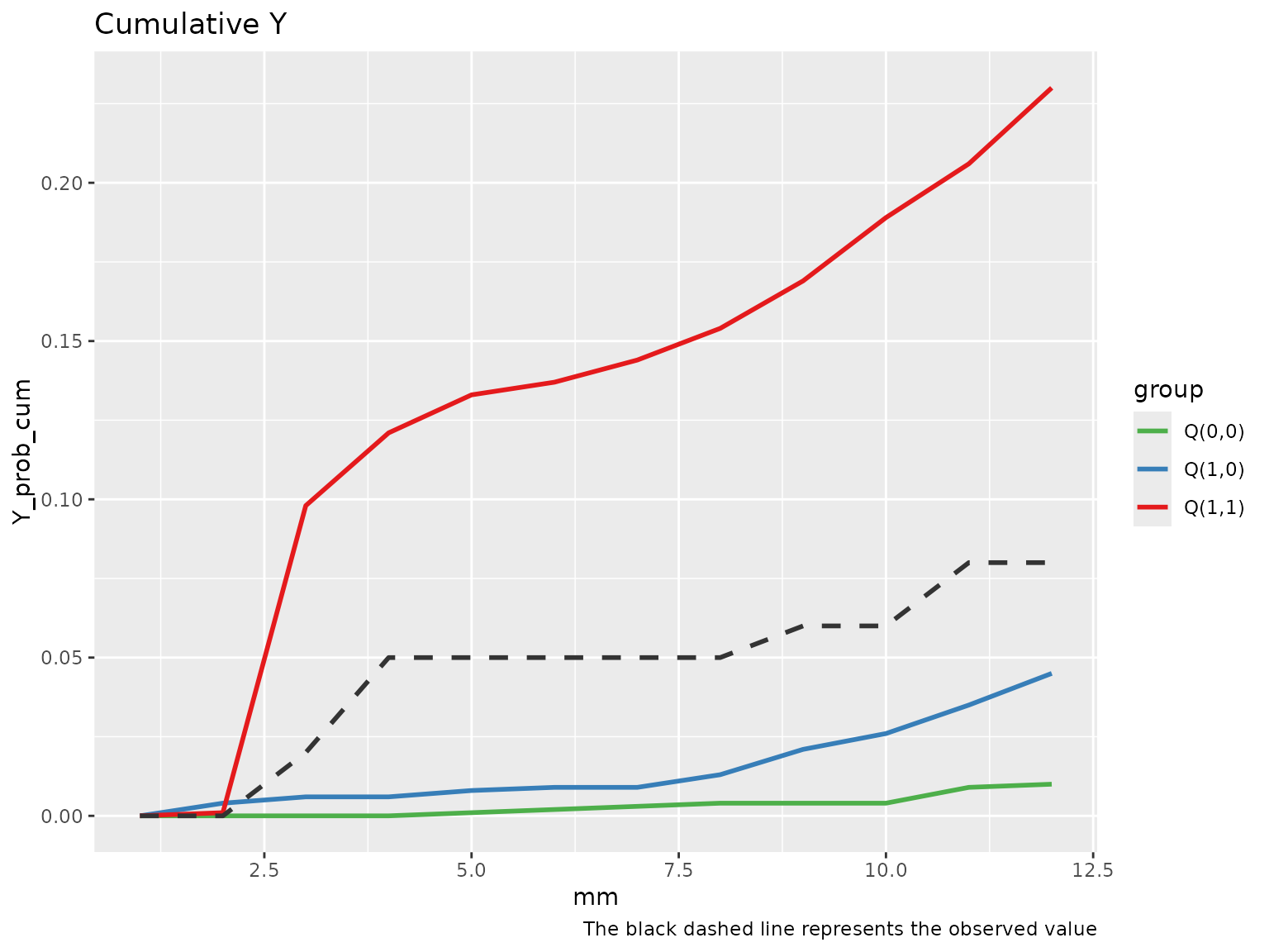
Diagnostic tools for checking the g-computation algorithm are limited. However, we should expect the observed outcome trajectory to lie between the predicted values of $Q(a, a)$ , $Q(a, a^*)$ , and $Q(a^*, a^*)$ over time.

To aid in this evaluation, tvmedg provides two diagnostic plots:

A plot comparing the observed outcome with the simulated outcomes under the three exposure–mediator scenarios across time.
A plot of the cumulative outcomes over time under each scenario.

Time-varying plot

plot(med_MtoL, "tvY")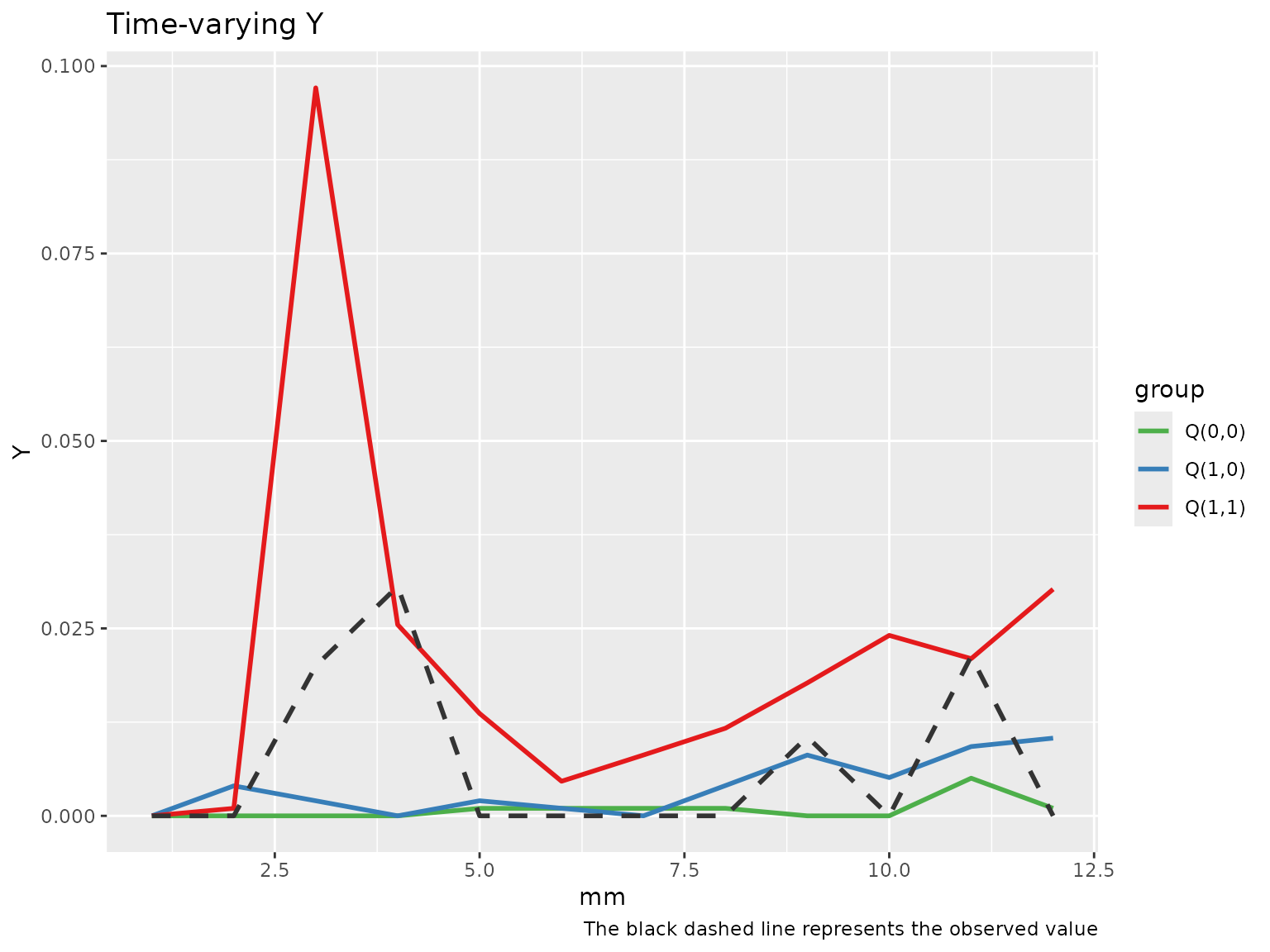

Cumulative plot

plot(med_MtoL, "cumY")